Pandas DataFrames

Learning Objectives

• Understand the advantages of using Pandas DataFrames.

• Be able to create a DataFrame by importing data or converting a dictionary.

• Be able to present, locate, filter and modify data within a DataFrame.

• Be able to use use DataFrame functions

Today we are going to look at a new Python library called Pandas. This library may be used when analysing more complex datasets.

---

Why use Pandas?

Up to this point in your degree it is likely that you have only worked with small data sets and that analysing your data has not posed too many challanges beyond those associated with learning a new skill. For this sort of work the methods and tools we have used to this point are more than sufficient, however as we begin to work with larger and more complex datasets, these methods may become inefficient and labourious - enter pandas. The key advantages of learning to use pandas are:

• Pandas is very useful for working with large amounts of data.

• Unlike numpy data does not have to be numeric.

• Data can be cleaned using pandas.

• Data can be filtered using pandas.

• Subsets of data can be extracted easily from a pandas dataframe.

• Pandas is used in data science.

One key disadvantage of using numpy is that it is unable to use categorical data (e.g. names, places, types, etc.) and instead can only deal with numbers. Take a look at the example data below and what happens when we try to feed it into numpy from a csv file:

Name	Age	Eye Colour	Height (m)
Joan	54	Brown	1.54
Davide	36	Blue	1.85
Liam	29	Hazel	1.74
Emily	28	Green	1.64
Carlos	15	Green	1.77
Katie	11	Blue	1.73
Ross	26	Blue	1.79
Zack	35	Hazel	1.55
Daisy	78	Brown	1.50
Kim	7	Blue	1.10
Schmonathan	68	Brown	1.68
Jamantha	57	Green	1.43
Carlos	20	Amber	1.91

[[  nan   nan   nan   nan]
 [  nan 54.     nan  1.54]
 [  nan 36.     nan  1.85]
 [  nan 29.     nan  1.74]
 [  nan 28.     nan  1.64]
 [  nan 15.     nan  1.77]
 [  nan 12.     nan  1.73]
 [  nan 26.     nan  1.79]
 [  nan 35.     nan  1.55]
 [  nan 78.     nan  1.5 ]
 [  nan  7.     nan  1.1 ]
 [  nan 68.     nan  1.68]
 [  nan 57.     nan  1.43]
 [  nan 20.     nan  1.91]]

It is clear that numpy is unable to be used when processing this data as it returns “nan” values (nan = not a number). Now let’s try using a pandas to import the same data:

	Name	Age	Eye Colour	Height (m)
0	Joan	54	Blue	1.54
1	Davide	36	Brown	1.85
2	Liam	29	Hazel	1.74
3	Emily	28	Green	1.64
4	Carlos	15	Green	1.77
5	Katie	12	Blue	1.73
6	Ross	26	Blue	1.79
7	Zack	35	Hazel	1.55
8	Daisy	78	Brown	1.50
9	Kim	7	Blue	1.10
10	Schmonathan	68	Brown	1.68
11	Jamantha	57	Green	1.43
12	Carlos	20	Amber	1.91

Pandas has not only been able to read in all of the data from the csv file, but it has also presented the data much more clearly. This is what we refer to as a DataFrame.

---

Creating A DataFrame from Scratch

It is often the case that rather than importing data into a DataFrame, we may just want to create one in our script. To do this is relatively simple, just take a look at the snippet of code below:

1. First I will create a dictionary containing information about various european countries.

2. Secondly, I will convert this into a pandas DataFrame.

Take a look at the lines of code below and ensure you understand how it is constructed.

# Creating my dictionary
euroData = {'Country': ['United Kingdom', 'Italy', 'France', 'Sweden', 'Finland', 'Malta', 'Germany'],
        'Capital City': ['London', 'Rome', 'Paris', 'Stockholm', 'Helsinki', 'Valletta', 'Berlin'],
        'Population': [67330000, 59110000, 67750000, 10420000, 5541000, 518536, 83200000],
        'Life Expectancy': [80.90, 82.34, 82.18, 82.41, 82.13, 82.65, 80.94]}

# Converting my dictionary into a pandas DataFrame
euroData = pd.DataFrame(data=euroData)
display(euroData)

	Country	Capital City	Population	Life Expectancy
0	United Kingdom	London	67330000	80.90
1	Italy	Rome	59110000	82.34
2	France	Paris	67750000	82.18
3	Sweden	Stockholm	10420000	82.41
4	Finland	Helsinki	5541000	82.13
5	Malta	Valletta	518536	82.65
6	Germany	Berlin	83200000	80.94

---

What can we do with a DataFrame?

Importing Data

Importing data using pandas is essentially the same as importing data using numpy:

• First, we will import pandas into the script in the same way we did for numpy.

• Next, use we use “read_csv” to import the data into a DataFrame.

import pandas as pd
Data = pd.read_csv("PeopleData.csv")

Getting to know our DataFrame

In order to get a feel for the data that we are working with, there are a few pandas commands we can use. We can look at our enitre DataFrame or just the top/bottom 5 rows of the DataFrame using appropriate commands.

# This is how we look at the entire DataFrame
display(Data)

	Name	Age	Eye Colour	Height (m)
0	Joan	54	Blue	1.54
1	Davide	36	Brown	1.85
2	Liam	29	Hazel	1.74
3	Emily	28	Green	1.64
4	Carlos	15	Green	1.77
5	Katie	12	Blue	1.73
6	Ross	26	Blue	1.79
7	Zack	35	Hazel	1.55
8	Daisy	78	Brown	1.50
9	Kim	7	Blue	1.10
10	Schmonathan	68	Brown	1.68
11	Jamantha	57	Green	1.43
12	Carlos	20	Amber	1.91

# This is how we take a look at the top 5 rows of the DataFrame.
Data.head()

	Name	Age	Eye Colour	Height (m)
0	Joan	54	Blue	1.54
1	Davide	36	Brown	1.85
2	Liam	29	Hazel	1.74
3	Emily	28	Green	1.64
4	Carlos	15	Green	1.77

# This is how we take a look at only select columns from the top 5 rows of the DataFrame.
Data[["Name", "Age"]].head()

	Name	Age
0	Joan	54
1	Davide	36
2	Liam	29
3	Emily	28
4	Carlos	15

# This is how we take a look at the bottom 5 rows of the DataFrame.
Data.tail()

	Name	Age	Eye Colour	Height (m)
8	Daisy	78	Brown	1.50
9	Kim	7	Blue	1.10
10	Schmonathan	68	Brown	1.68
11	Jamantha	57	Green	1.43
12	Carlos	20	Amber	1.91

# This is how we take a look at only select columns from the bottom 5 rows of the DataFrame.
Data[["Name", "Age"]].tail()

	Name	Age
8	Daisy	78
9	Kim	7
10	Schmonathan	68
11	Jamantha	57
12	Carlos	20

We are also able to gauge properties of the DataFrame such as what the each column represents, the types of data that it contains, the shape of the DataFrame and information about the indexing:

1. An example of how to find out what information is contained in each column:

print(Data.columns)

Index(['Name', 'Age', 'Eye Colour', 'Height (m)'], dtype='object')

2. An example of how to find out what type of data is stored in the DataFrame:

print(Data.dtypes)

Name           object
Age             int64
Eye Colour     object
Height (m)    float64
dtype: object

3. An example of how to find out what the shape of the DataFrame is:

print(Data.shape)

(13, 4)

4. An example of how to find out the indexing of the DataFrame:

print(Data.index)

RangeIndex(start=0, stop=13, step=1)

5. To look at specific entries in a DataFrame we can use the “.loc” and “.iloc” functions.

When using loc we are specifying which entry in the DataFrame we want using the index labels, whereas iloc uses the index positions. If our index labels are just our index positions, there will be no difference when using loc or iloc bar the fact that loc gives an inclusive range of results whereas iloc gives an exlusive range of results.

Make sure this is clear to you by reviewing the difference in the outputs from the snippets of code below:

# Using loc
print(Data.loc[0], "\n \n")
print(Data.loc[0:0], "\n \n")
print(Data.loc[0:3], "\n \n")
print(Data.loc[0][2])

# If we had added an alternative index to the data frame that did not begin at zero
# e.g. (101, 102, 103, ...) we would use these values when using loc.

Name          Joan
Age             54
Eye Colour    Blue
Height (m)    1.54
Name: 0, dtype: object 
 

   Name  Age Eye Colour  Height (m)
0  Joan   54       Blue        1.54 
 

     Name  Age Eye Colour  Height (m)
0    Joan   54       Blue        1.54
1  Davide   36      Brown        1.85
2    Liam   29      Hazel        1.74
3   Emily   28      Green        1.64 
 

Blue

# Using iloc
print(Data.iloc[0], "\n \n")
print(Data.iloc[0:0], "\n \n")
print(Data.iloc[0:3], "\n \n")
print(Data.iloc[0][2])

# If we had added an alternative index to the data frame that did not begin at zero
# e.g. (101, 102, 103, ...) we would still use the index location (e.g. 0, 1, 2).

Name          Joan
Age             54
Eye Colour    Blue
Height (m)    1.54
Name: 0, dtype: object 
 

Empty DataFrame
Columns: [Name, Age, Eye Colour, Height (m)]
Index: [] 
 

     Name  Age Eye Colour  Height (m)
0    Joan   54       Blue        1.54
1  Davide   36      Brown        1.85
2    Liam   29      Hazel        1.74 
 

Blue

Filtering Data

It is often the case when working with large datasets that we are only actually interested in a subset of the data. For example, using the “Data” DataFrame above I may only want to see the heights of the participants in this particular study. To this I can simply filter this information from the DataFrame:

Heights = Data["Height (m)"]
print(Heights)

0     1.54
1     1.85
2     1.74
3     1.64
4     1.77
5     1.73
6     1.79
7     1.55
8     1.50
9     1.10
10    1.68
11    1.43
12    1.91
Name: Height (m), dtype: float64

In the example above I have created a new DataFrame containing just the heights that I may then use in my analysis moving forward. This saves me having to extracting the information from the larger DataFrame everytime that information is required. Either method is fine.

We can see that when the “Heights” DataFrame has been printed out that the index is also shown. If we would like to extract a particular value from the DataFrame we can do so using the index:

selectedHeight = Heights[6]
print(selectedHeight)

1.79

In the example above “selectedHeight” was extracted from the DataFrame “Heights” in the same way that we would extract information from a numpy array or list. If we wanted to select this Height from the original larger DataFrame “Data”, we would simply use two sets of square brackets:

selectedHeight = Data["Height (m)"][6]
print(selectedHeight)

1.79

In some instances it may be useful to know all of the unique values in your DataFrame. For example, perhaps from my sample of data I would like to know all of the unique eye colours of the people that were sampled:

UniqueEyeColours = Data["Eye Colour"].unique()
print(UniqueEyeColours)

['Blue' 'Brown' 'Hazel' 'Green' 'Amber']

Or perhaps I just want to the information relating to one of the particpants in my survey. Look carefully at the structure of the line of code below used to extract the information associated with Carlos:

CarlosInfo = Data[Data["Name"] == 'Carlos']
print(CarlosInfo)

      Name  Age Eye Colour  Height (m)
4   Carlos   15      Green        1.77
12  Carlos   20      Amber        1.91

As there are two people named Carlos in my data I have been presented with two rows of data. If I want to filter the data to be even more specific I simply add a second condition in the filtering command.

I am specifically interested in the data associated with the Carlos with amber eyes. I will add a second critereon to be met in the filtering using “&”. Note that each condition is enclosed in a pair of rounded brackets. Look at the code below closely:

CarlosInfo = Data[(Data["Name"] == 'Carlos') & (Data["Eye Colour"] == 'Amber')]
print(CarlosInfo)

      Name  Age Eye Colour  Height (m)
12  Carlos   20      Amber        1.91

If I want to get data for people called Carlos or Katie, I can simply modify the code above by adding an “or” statement using “|”:

NewData = Data[(Data["Name"] == 'Carlos') | (Data["Name"] == 'Katie')]
print(NewData)

      Name  Age Eye Colour  Height (m)
4   Carlos   15      Green        1.77
5    Katie   12       Blue        1.73
12  Carlos   20      Amber        1.91

If I want to filter my data to only show those who are taller than 1.8m I can do so by applying a condition:

TallPeople = Data[(Data["Height (m)"] > 1.8)]
print(TallPeople)

      Name  Age Eye Colour  Height (m)
1   Davide   36      Brown        1.85
12  Carlos   20      Amber        1.91

Replacing Data

It might be the case that there is an incorrect data entry in a DataFrame that needs correcting, or perhaps a series of terms all need replacing. We can easily replace terms in a DataFrame using “.replace()”. For example, lets say that the age recorded for Davide was incorrect and needed replacing, we can do so easily. Here I am going to replace the number 36 with 38 in the age column.

Data['Age'] = Data["Age"].replace([36],38)
Data.head()

	Name	Age	Eye Colour	Height (m)
0	Joan	54	Blue	1.54
1	Davide	38	Brown	1.85
2	Liam	29	Hazel	1.74
3	Emily	28	Green	1.64
4	Carlos	15	Green	1.77

Replacing all values equal to something thing can be useful, but may also result in data being changed that should not be changed. For example, when correcting the age of Davide above, the method would actually have re-aged anybody who is 36 to 38.

If we want to change an individual value we can also do this fairly easily too. Take a look at the example below where I am going to change the eye colour associated with Liam from Hazel to Amber:

Data.iloc[2,2] = "Amber"
Data.head()

	Name	Age	Eye Colour	Height (m)
0	Joan	54	Blue	1.54
1	Davide	38	Brown	1.85
2	Liam	29	Amber	1.74
3	Emily	28	Green	1.64
4	Carlos	15	Green	1.77

Looping

In addition to filtering data from a DataFrame, it is also possible to perform calculations/analysis by looping through it (e.g. using for and while loops).

To show an example of how we can loop through a DataFrame we are going to use a new set of data called “all_matches”. This dataset contains the results of all international football matches from 1872 to 2023. We are going to loop through this data to determine which country is the most successful of all time:

1. The first thing we should do is take a look at how the data in the DataFrame is formatted. To do this, we will use “.head()” to view the first five rows of the DataFrame.

import matplotlib.pyplot as plt
Football = pd.read_csv("all_matches.csv")

Football.head()

	date	home_team	away_team	home_score	away_score	tournament	country	neutral
0	1872-11-30	Scotland	England	0	0	Friendly	Scotland	False
1	1873-03-08	England	Scotland	4	2	Friendly	England	False
2	1874-03-07	Scotland	England	2	1	Friendly	Scotland	False
3	1875-03-06	England	Scotland	2	2	Friendly	England	False
4	1876-03-04	Scotland	England	3	0	Friendly	Scotland	False

2. Next, in order to determine which country is the most successful we need to know how many different countries are actually in this dataset. When doing this I will assume that every team has played at home and away. To do this, we can use “.unique()” as above:

countries = Football["home_team"].unique()
print(countries)

['Scotland' 'England' 'Wales' 'Ireland' 'Uruguay' 'Austria' 'Hungary'
 'Argentina' 'Belgium' 'France' 'Netherlands' 'British Guiana' 'Bohemia'
 'Switzerland' 'Germany' 'Sweden' 'Denmark' 'Italy' 'South Africa' 'Chile'
 'Norway' 'Finland' 'Luxembourg' 'Russia' 'Philippines' 'China' 'Suriname'
 'Brazil' 'Japan' 'Paraguay' 'Spain' 'Czechoslovakia' 'Egypt'
 'Northern Ireland' 'Estonia' 'Costa Rica' 'Guatemala' 'Poland'
 'Yugoslavia' 'New Zealand' 'Romania' 'Latvia' 'Portugal' 'Australia'
 'Lithuania' 'Trinidad and Tobago' 'Turkey' 'Mexico' 'Aruba'
 'United States' 'Soviet Union' 'Haiti' 'Bulgaria' 'Canada' 'Jamaica'
 'Kenya' 'Azerbaijan' 'Georgia' 'Peru' 'Honduras' 'British Honduras'
 'Dutch East Indies' 'El Salvador' 'Uganda' 'Barbados' 'Greece' 'Cuba'
 'Curaçao' 'Faroe Islands' 'Mauritius' 'Dominica' 'Reunion'
 'New Caledonia' 'Palestine' 'Grenada' 'Guadeloupe' 'French Guiana'
 'Martinique' 'St Vincent & Grenadines' 'Panama' 'Colombia' 'Venezuela'
 'Bolivia' 'Saint Kitts and Nevis' 'Ecuador' 'Slovakia'
 'Bohemia and Moravia' 'Croatia' 'Iran' 'Afghanistan' 'Korea' 'Lebanon'
 'Syria' 'Nicaragua' 'Iceland' 'Albania' 'Southern Rhodesia' 'Hong Kong'
 'Tanganyika' 'French Somaliland' 'Northern Rhodesia' 'Madagascar'
 'South Vietnam' 'Macao' 'Singapore' 'India' 'South Korea' 'Thailand'
 'Belgian Congo' 'Ethiopia' 'Puerto Rico' 'Israel' 'Sierra Leone'
 'Zanzibar' 'Antigua and Barbuda' 'Saint Kitts' 'Netherlands Antilles'
 'Gold Coast' 'West Germany' 'Indonesia' 'East Germany' 'Fiji' 'Nigeria'
 'Montserrat' 'Ceylon' 'Pakistan' 'Tahiti' 'Saar' 'Gambia'
 'Portuguese Guinea' 'Jordan' 'Libya' 'New Hebrides' 'Burma' 'Taiwan'
 'French Togoland' 'Ivory Coast' 'French Congo' 'Cameroon' 'Malaya'
 'Cambodia' 'Sudan' 'North Korea' 'Ubangi-Shari' 'Malta' 'Tunisia' 'Iraq'
 'Morocco' 'Saudi Arabia' 'Ghana' 'Nyasaland' 'Algeria'
 'United Arab Republic' 'Dahomey' 'North Vietnam' 'Togo' 'Congo'
 'Mali Federation' 'Upper Volta' 'Cyprus' 'Saint Lucia' 'Kuwait' 'Senegal'
 'Liberia' 'Central African Republic' 'Chad' 'Guinea' 'Mali' 'Gabon'
 'Northern Cyprus' 'Congo-Leopoldville' 'Solomon Islands' 'Malaysia'
 'Niger' 'DR Congo' 'Bermuda' 'Tanzania' 'Zambia' 'Bahrain' 'Malawi'
 'Papua New Guinea' 'Dominican Republic' 'Guyana' 'Mauritania' 'Rhodesia'
 'Swaziland' 'Laos' 'Qatar' 'Bonaire' 'Khmer Republic' 'Lesotho' 'Bahamas'
 'South Yemen' 'Somalia' 'Zaire' 'United Arab Emirates' 'Sri Lanka'
 'Nepal' 'Bangladesh' 'Burundi' 'Guinea-Bissau' 'Mozambique' 'Guam'
 'Angola' 'Oman' 'São Tomé and Príncipe' 'Botswana' 'Benin' 'Cape Verde'
 'Seychelles' 'Rwanda' 'Comoros' 'Tuvalu' 'Wallis and Futuna' 'Tonga'
 'Kiribati' 'Brunei' 'Zimbabwe' 'Liechtenstein' 'Vanuatu' 'Greenland'
 'Western Samoa' 'Eastern Samoa' 'Belize' 'Djibouti' 'Maldives'
 'Burkina Faso' 'North Yemen' 'Anguilla' 'Equatorial Guinea'
 'Cayman Islands' 'Sint Maarten' 'Namibia' 'Saint Martin'
 'British Virgin Islands' 'San Marino' 'Slovenia' 'Moldova'
 'Comm of Indep States' 'Ukraine' 'Kazakhstan' 'Tajikistan' 'Uzbekistan'
 'Eritrea' 'Turkmenistan' 'Kyrgyzstan' 'Armenia' 'Belarus' 'Vietnam'
 'Yemen' 'Myanmar' 'Macedonia' 'Czechia' 'Gibraltar' 'Cook Islands'
 'Bosnia and Herzegovina' 'Andorra' 'US Virgin Islands' 'Palau'
 'Northern Mariana Islands' 'Samoa' 'Turks and Caicos Islands'
 'FS Micronesia' 'Mayotte' 'Bhutan' 'Kosovo' 'Serbia and Montenegro'
 'Mongolia' 'Serbia' 'Montenegro' 'Kurdistan' 'South Sudan'
 'Saint Barthelemy' 'East Timor' 'Eswatini' 'North Macedonia']

3. Now we have a list off all the countries we need to extract data for, we can loop through the entire data set and determine how many matches each country has won. This is made a little more complicated as looking at the data we need to consider both the home and away games:

# First we create two lists - one for the country name and one for their percentage of wins.
teamNames = []
percentageWins = []

for country in countries:
    
    # First we will filter only the data associated with our current country from the entire dataset.
    # This first line of code narrows down the data to only the matches where they were either playing home or away.
    currentCountry = Football[(Football['home_team']==country) | (Football['away_team']==country)]
    
    # This line of code simply filters from the currentCountry DataFrame to determine how many home wins they had.
    HomeWins = currentCountry[(currentCountry['home_team'] == country) & (currentCountry['home_score'] > currentCountry['away_score'])]
    # This line of code simply filters from the currentCountry DataFrame to determine how many away wins they had.
    AwayWins = currentCountry[(currentCountry['away_team'] == country) & (currentCountry['away_score'] > currentCountry['home_score'])]
    
    # Now we calculate the number of wins as a percentage and append our data to our two lists.
    teamNames.append(country)
    percentageWins.append( ((HomeWins.shape[0] + AwayWins.shape[0]) / currentCountry.shape[0]) * 100 ) 
    # In the line above the number of home wins, away wins and games played is determined using .shape[0]

4. I will now create a new DataFrame containing the countries and their win percentage from the lists I made in the last step:

# Building my new DataFrame
winData = pd.DataFrame({'Country Name': teamNames, 'Percentage Wins': percentageWins})

# Printing the top 5 rows of my DataFrame
winData.head()

	Country Name	Percentage Wins
0	Scotland	47.738095
1	England	58.451957
2	Wales	31.926864
3	Ireland	35.104895
4	Uruguay	44.308943

5. I can sort our new DataFrame by the column “Percentage of Wins” to determine the country that is the most successful:

# Sorting the values by most sucessful
sortedWinData = winData.sort_values('Percentage Wins', ascending=False)
sortedWinData.head()

	Country Name	Percentage Wins
143	Ubangi-Shari	100.000000
137	French Congo	100.000000
90	Korea	100.000000
157	Mali Federation	75.000000
115	Saint Kitts	72.727273

Plotting Data from a DataFrame

6. If I want to visualise this data in a better way that a simple table, we can also extract the data from a DataFrame for plotting. The process is exactly the same as if we were plotting data from a numpy array. For example the bar chart below shows the 20 most successful countries at football:

import matplotlib.pyplot as plt

plt.figure(figsize = (8,7))
plt.bar(sortedWinData['Country Name'][0:20], sortedWinData['Percentage Wins'][0:20])
plt.ylabel("Percentage Wins")
plt.xlabel("Country")
plt.title("Most Successful Countries @ Football")
plt.xticks(rotation = 90)
plt.show()

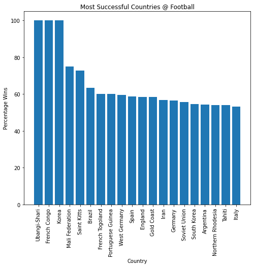
There we have it! The most successful countries of all time at football are Ubangi-Shari (a former French colony in Africa), French Congo (former French colony) and Korea (before the seperation of states). Let’s take a look at their record by filtering our original Football DataFrame to show only these countries matches:

TopTeams = Football[(Football["country"] == "Ubangi-Shari") | 
                   (Football["country"] == "French Congo") | 
                   (Football["country"] == "Korea") ]
TopTeams.head()

	date	home_team	away_team	home_score	away_score	tournament	country	neutral
2812	1942-08-16	Korea	Japan	5	0	Friendly	Korea	False
4322	1954-12-31	French Congo	Cameroon	5	1	Friendly	French Congo	False
4715	1956-12-31	Ubangi-Shari	Cameroon	5	1	Friendly	Ubangi-Shari	False

Each team only played (and won) a single match before, but I am inclined to give Korea the crown as they had the largest goal difference… So there we have it - Korea is the greatest football nation on the planet!

---

Useful Pandas DataFrame Functions

There are lots of very useful pandas specfic functions - those related to DataFrames can be found here.

---

Activities

1. Brazil vs Portugal

Using “all_matches.csv” find out the following:

• How many football games have been played between Brazil and Portugal.

• Who has won the most when playing each other.

• Who has won the most games overall (i.e. not just against each other).

2. Learning = Earning?

Using the “BankChurners.csv” data:

• Use a for loop to determine the mean credit limit for each education level in the data.

• Plot the mean credit limit for each education level in the data.

• Plot the mean utilisation ration for each education level in the data.

You will want to use .mean() for this activity. If you use the .mean() method it will return mean for all the columns, you will need to select the column you are interested in.

3. “The price of greatness is responsibility.”

Using the “politics_apr2020.csv” data:

• Print the countries with the youngest leaders.

• Print the countries with the oldest leaders.

• Find the longest serving leader.

• Plot the leaders against tenure.

4. Covid-19

Using the “covid19_stats.csv” data:

• Calculate the total number of excess deaths attributed to Covid-19 for each country in 2021.

• Show the top and bottom 5 countries by excess deaths.

• Plot the total number of deaths attributed to covid.

5. Global Statistics

Using the “global_stats.csv” data:

• Determine how many different countries can be found within each continental base in this dataset.

• Print out the top/bottom 5 populated countries within each continental base.

• Rank and plot the Human development Index (HDI) for countries with more than 50 million internet users.